If you know about Uniswap V2, you definitely know that its biggest advantage is “fully automated,” and its biggest problem is also “fully automated.” Once funds enter, they are mechanically distributed across the entire price range from 0 to ∞.
This is supposed to be fair, but extremely inefficient:
Most of the time, assets are “sleeping” far away from the current market price, nobody trades there, and no fees are generated.
Therefore, Uniswap V3 proposed a revolutionary concept: Concentrated Liquidity.
It allows LPs to “concentrate” capital within the price range they consider appropriate so that “active money actually works.”
I. What is Concentrated Liquidity: Background and the Problem It Solves
The decentralized trading protocol Uniswap uses the automated market maker (AMM) model. Users don’t need to place orders or find counterparties — simply deposit two tokens into a pool to become a liquidity provider. This model is very simple, but it also brings an unnoticed problem: most liquidity does not actually work.
To illustrate this, we need to review the mechanism of Uniswap v2.
1. Traditional AMM: Constant Product and “Full Price Range”
In v2’s constant product model, a trading pool maintains a formula:
x · y = k
Here, x and y are the quantities of two assets in the pool, and k is a constant. No matter how the price fluctuates, this formula always holds.
But the model implicitly assumes:
The liquidity of the pool is distributed across the entire price range from 0 to ∞.
Theoretically, no matter how high or low the price goes, the pool is “ready” to provide liquidity.
The problem: real prices never go to 0 or infinity.
In other words, liquidity is passively spread across a ridiculously wide range that will almost never be used.
2. Liquidity Utilization Problems
Distributing liquidity across an overly wide range results in a very direct consequence:
Most capital is sleeping.
In reality, prices tend to fluctuate within a narrow band, so only funds inside that range actually participate in trades. Other funds are just lying around, consuming capital efficiency.
This leads to two impacts:
- For traders, active depth is limited, causing higher slippage
- For LPs, although much capital is locked, the return is not proportional
In other words:
Capital utilization is low.
3. Why Concentrated Liquidity Is Needed
Uniswap v3 introduces Concentrated Liquidity, with the following core idea:
Liquidity should be placed where actual trading happens.
If the price stays in a certain region for a long time, LPs can concentrate liquidity in that region instead of wasting it on extreme prices that might never occur.
The effects are significant:
- The same capital provides deeper liquidity
- Price impact for large orders is reduced
- Fee revenue increases
This essentially changes the AMM from “broad distribution” to “locally effective distribution.”
4. Definition of Concentrated Liquidity
Strictly speaking, Concentrated Liquidity means:
LPs only provide liquidity within a self-defined price range \([P_{lower}, P_{upper}]\). Once price moves outside the range, the LP stops participating and stops earning fees.
That means each LP is no longer just part of a pool, but becomes a “conditional liquidity position.”
From the contract’s perspective, the large pool is divided into many segments, and liquidity is placed into each range. Whichever range trades happen within, LPs of that segment earn fees.
5. What Problem Does It Actually Solve
In one sentence:
Use the same capital to obtain deeper effective liquidity.
But specifically, it improves three things:
- Capital Efficiency
- Lower Slippage
- Higher Fee Yield
These all come from one fact: liquidity can finally be concentrated rather than being infinitely diluted.
6. But It’s Not a Free Optimization
Concentrated liquidity does not change the basic AMM logic but introduces a new dimension: price range.
This makes the LP role more strategic, similar to predicting price movement. Therefore, it also introduces a new risk:
- If price moves out of the chosen range, the position becomes single-sided and stops earning.
To earn more, LPs must take on more management and judgement — a typical risk-return tradeoff.
II. How Concentrated Liquidity Works
1. Inputs Required to Provide Liquidity
Suppose we provide liquidity into an ETH/USDC pool, the contract requires:
-
Token pair: ETH / USDC
-
Price range
- lower price example: 2000 USDC/ETH
- upper price example: 3000 USDC/ETH
-
Amount of ETH or USDC provided
In other words, we’re telling the contract three things:
- I want to LP for ETH/USDC
- Within 2000–3000
- I’m willing to deposit this amount of tokens
2. Which Token(s) Must Be Deposited
Suppose current ETH/USDC price is 2500, then the system checks:
2000 < 2500 < 3000
Meaning “price is inside the range.”
This is extremely important because it determines which assets we need to provide:
Three situations
| Current Price | Required Deposit |
|---|---|
| Inside range | Provide both ETH and USDC |
| Below range | Only USDC |
| Above range | Only ETH |
Why? Not strategy — pure math: AMM models automatically bias towards one asset depending on price.
Simply put, scarcity determines demand. At low price, the pool needs more USDC; at high price, more ETH.
3. Understanding Liquidity (L)
Although we deposit ETH/USDC, the contract records a variable L (liquidity unit).
Key points:
- We deposit assets
- Contract records L
- Earnings are proportional to L
In short:
L is our “position size” in that price range.
The amounts of ETH/USDC adjust automatically with price.
4. Price Range Discretization
We enter ranges in continuous price (e.g., 2000–3000), but internally the contract uses ticks.
It converts them to:
- \(tick_{Lower}\)
- \(tick_{Upper}\)
Ticks discretize price boundaries.
The contract then stores only boundary updates:
- add +L at \(tick_{Lower}\)
- subtract –L at \(tick_{Upper}\)
Active liquidity at current price equals the sum of all netLiquidity values below the current tick.
For example, if \(tick_{Lower}=100\) and \(tick_{Upper}=200\), the contract records:
netLiquidity[100] += 10
netLiquidity[200] -= 10
If the current price tick is 150, the activeLiquidity equals the sum of all netLiquidity where tick < 150, which is 10.
If the current price tick is 205, then activeLiquidity equals the sum of all netLiquidity where tick < 205, which is 0.
Therefore, when the price crosses these ticks, the system knows when to start and when to stop using our liquidity.
Why do we need to discretize price when storing ranges?
If we simply used linear segmentation, such as slicing the 2000–3000 range into 1000 parts, each worth 1 USDC, it would seem natural.
But what if the price range becomes 0.2–0.3 or even lower? If we still slice it into 1000 segments, each segment would become extremely small, and the overall scale would be highly uneven.
Furthermore, real token prices can span multiple orders of magnitude, from 0.0000001 to 10,000,000, making uniform segmentation impossible.
How do we perform discretization?
We define that each tick corresponds to a price that is a fixed multiple \(r\) of the previous tick. Then, for \(tick+1\), the price \(P_{tick+1}\) satisfies:
\[ P_{tick+1} = P_{tick} \times r \]From which we derive:
\[ P_{tick} = P_0 \times r^{tick} \]If we set \(P_0 = 1\) and \(r=1.0001\), then:
\[ P_{tick} = 1.0001^{tick} \]This means each tick movement corresponds to a 0.01% price change.
Now we can represent any price using ticks:
\[ tick = \log_{1.0001}(P) \]For example:
\(P = 0.25\) corresponds to \(tick \approx -13864\)
\(P = 2500\) corresponds to \(tick \approx 78244\)
Thus, we obtain a uniform tick scale that works for arbitrary token prices (as long as they’re not negative 🤪)
5. Storing Liquidity State
When we add liquidity, the system issues an NFT that records:
- chosen price range (2000–3000)
- size of L
- accumulated fees claimable
- current fee status required for future fee calculations
Therefore:
The LP action is no longer part of the pool itself, but an independent position recorded as an NFT.
6. Position Changes
When price is within the range:
- holds both ETH and USDC
- converts between the two as trades occur
- participates in matching and earns fees
If price falls below 2000:
- position becomes entirely USDC
- no longer provides liquidity or earns fees
If price exceeds 3000:
- position becomes entirely ETH
- also exits liquidity
In other words:
When ETH rises, the position becomes ETH-heavy; when ETH falls, it becomes USDC-heavy.
This behavior is not a strategy — it is automatically done by the AMM logic.
7. Fee Settlement
When trades occur inside the range (2500 is inside), fees accumulate. Internally, the contract records fees in the feeGrowth variable.
When withdrawing, the contract does two things:
- returns current holdings (could be ETH+USDC or single-token)
- returns accumulated fees
No need to manually claim—withdrawal automatically settles everything.
III. Main Formula Derivations
1. Official Whitepapers
v2: https://docs.uniswap.org/whitepaper.pdf
v3: https://app.uniswap.org/whitepaper-v3.pdf
v4: https://app.uniswap.org/whitepaper-v4.pdf
2. Basic Formulas
Virtual reserve curve (trading model):
\[ x \times y = k \tag{1} \]Liquidity:
\[ L = \sqrt{xy} \tag{2} \]Price:
\[ P = \frac{y}{x} \tag{3} \]Effective reserve curve:
\[ (x+\dfrac{L}{\sqrt{p_{b}}})(y+L\sqrt{p_{a}})=L^{2} \tag{4} \]2. Derivation of the Effective Reserve Curve
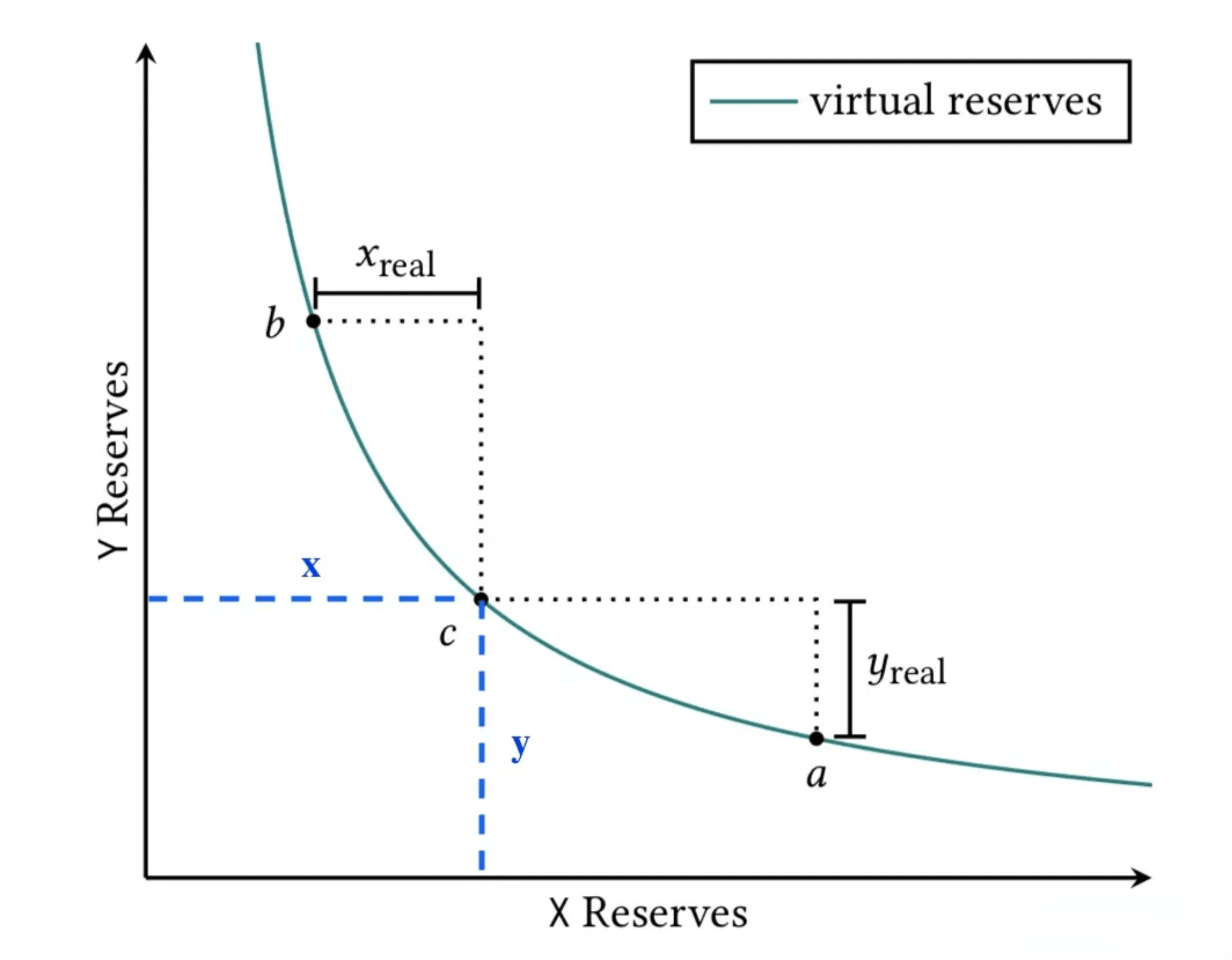
As shown in Figure 1, the current price is at point c. Suppose the actual price movement range is \([a,b]\).
When the price moves from c to a, the maximum pool consumption for token \(y\) is \(y_{real}\). Likewise, when price moves from c to b, the maximum pool consumption for token \(x\) is \(x_{real}\).
Therefore, in theory, only \(x_{real}\) and \(y_{real}\) are required. All other funds are permanently unused, which also explains why the original xyk model has low capital efficiency.
So the question is: what should the effective reserve curve actually look like?
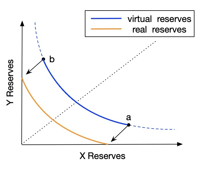
As shown in Figure 2, we begin deriving the effective reserve curve.
From the following formulas:
\[ L^2 = xy \\ P = \frac{y}{x} \]For anyone who has attended junior high school mathematics, multiplying and dividing both sides of the equations easily yields:
\[ \begin{aligned} x = \dfrac{L}{\sqrt{P}} \\ y = L\sqrt{P} \tag{4} \end{aligned} \]From Figure 1 we know:
\[ x = x_{real} + x_b \\ y = y_{real} + y_a \]Substituting into the xyk model (1):
\[ (x_{real}+x_b)(y_{real}+y_a) = k = L^2 \]Then substituting \(x_b, y_a\) using formula (4):
\[ (x_{real}+\dfrac{L}{\sqrt{P_{b}}})(y_{real}+L\sqrt{P_{a}})=L^{2} \]This is the final formula of the effective reserve curve.
3. Calculating Liquidity Composition Changes
After we provide liquidity, the contract starts performing trades. So how do we calculate the current allocation of assets inside our provided liquidity?
Based on formula (4):
\[ \begin{aligned} x=\dfrac{L}{\sqrt{p}} \\ y=L\sqrt{P} \tag{4} \end{aligned} \]Let:
\[ \begin{aligned} S = \sqrt{P} \end{aligned} \]Then:
\[ \begin{aligned} x = \dfrac{L}{S} \\ y = L S \end{aligned} \]Since L remains constant, differentiate with respect to S:
For x:
\[ x = \frac{L}{S} \Rightarrow dx = -L \frac{1}{S^2} dS \]For y:
\[ y = L S \Rightarrow dy = L dS \]So we have two important differential relationships:
\[ dx = -L \frac{1}{S^2} dS,\qquad dy = L dS \]Suppose an LP’s effective price range is:
- Lower price: \(P_a\), corresponding to \(S_a = \sqrt{P_a}\)
- Upper price: \(P_b\), corresponding to \(S_b = \sqrt{P_b}\)
Consider only the \(token_y\) change
Inside the range, when S increases from \(S_a\) to \(S_b\):
\[ dy = L dS \]Integrate S from \(S_a\) to \(S_b\):
\[ \Delta y = \int_{S_a}^{S_b} L\, dS = L (S_b - S_a) = L(\sqrt{P_b} - \sqrt{P_a}) \]This is the total amount of \(token_y\) corresponding to the entire interval \([P_a, P_b]\):
\[ amount_y = L(\sqrt{P_b} - \sqrt{P_a}) \]Consider only \(token_x\)
\[ dx = -L \frac{1}{S^2} dS \]Note that x decreases as S increases (price rises → token_x decreases). We want the total amount in absolute value:
\[ \Delta x = \int_{S_a}^{S_b} L \frac{1}{S^2} dS \]Compute:
\[ \int \frac{1}{S^2} dS = -\frac{1}{S} \]Thus:
\[ \Delta x = L\left[-\frac{1}{S}\right]_{S_a}^{S_b} = L\left(-\frac{1}{S_b} + \frac{1}{S_a}\right) = L\left(\frac{1}{S_a} - \frac{1}{S_b}\right) \]Substitute \(S = \sqrt{P}\):
\[ amount_x = L\left(\frac{1}{\sqrt{P_a}} - \frac{1}{\sqrt{P_b}}\right) \]This is the interval formula for \(token_x\).
The above derivation covers total x/y in the entire interval \([P_a, P_b]\). But the actual situation depends on where the current price lies:
Case A: Current price inside the range \((P_a < P < P_b)\)
The position holds “part token0 and part token1”:
-
For \(token_x\), effective interval is [P, P_b]:
\[ amount_x = L\left(\frac{1}{\sqrt{P}} - \frac{1}{\sqrt{P_b}}\right) \] -
For \(token_y\), effective interval is [P_a, P]:
\[ amount_y = L(\sqrt{P} - \sqrt{P_a}) \]
Case B: Price below the range \((P \le P_a)\)
The position has not “moved upward yet,” and is entirely in \(token_x\):
\[ amount_x = L\left(\frac{1}{\sqrt{P_a}} - \frac{1}{\sqrt{P_b}}\right) \\ amount_y = 0 \]Case C: Price above the range \((P \ge P_b)\)
The position has “fully moved upward,” and is entirely \(token_y\):
\[ amount_x = 0 \\ amount_y = L(\sqrt{P_b} - \sqrt{P_a}) \]4. Calculating the Actual Trading Price
Now that we understand the trading principle and core formulas, when preparing to swap tokens through the pool, the assets we input will also affect the ratio between pool assets. Since \(P=\dfrac{y}{x}\) is only a theoretical price, how do we calculate the actual execution price? For example, how many USDC can 1 ETH be swapped for?
When we put \(\Delta x\) ETH into the pool, USDC in the pool decreases by \(\Delta y\), and the corresponding price moves from \(P_0\) down to \(P_1\). So we have:
\[ \begin{aligned} \Delta x &= L\left(\frac{1}{\sqrt{P_1}} - \frac{1}{\sqrt{P_0}}\right) = L\left(\frac{1}{S_1} - \frac{1}{S_0}\right) \Rightarrow S_1 = \frac{1}{\dfrac{\Delta x}{L} + \dfrac{1}{S_0}} \\ \Delta y &= L(\sqrt{P_0} - \sqrt{P_1}) = L(S_0 - S_1) = L\left(S_0 - \frac{1}{\dfrac{\Delta x}{L} + \dfrac{1}{S_0}}\right) \end{aligned} \]where L is the active liquidity in the current price segment.
If the trade size is large and crosses multiple ticks, split the swap into segments and apply the same method for each interval, summing all the Δy values across each segment.